Preprocessing for Time Series

Note that a variation on this article may also be posted on the Nousot blog.

Time series are a string of numbers varying across time. It could be the weather, sales of tissue paper, electricity demand of a region, or countless other things. There are plenty of useful things to do with this type of data, but here, the focus is on forecasting: predicting the future values of these series for the purpose of guiding decision making.

Almost all time series forecasting begins by considering that the series in question represents two basic elements, the signal and the noise. The signal is the underlying pattern we seek to predict, and the noise are random events such as errors in the recordings of the data. Preprocessing of time series data can include many adjustments, but is largely, and for our purposes here, entirely, focused on removing the noise so that the underlying signal is easier for models to predict.

However, to really understand what is to be done, it is important to realize that there really is no such thing as “useless noise” but rather primary signals and secondary signals. For example, sales data may be primarily driven by a weekday signal (highest sales on Saturday, for instance) and a yearly signal (highest during Christmas shopping) but then also has a mixture of global events, national events, local events, promotions, competitor marketing, weather, construction near stores, and so on infinitely which all together produce the final sales on any particular day. Which of these are the primary signals depends mostly on the availability of quality data, the amount of effort expected for the forecasting project, and the final model to be used.

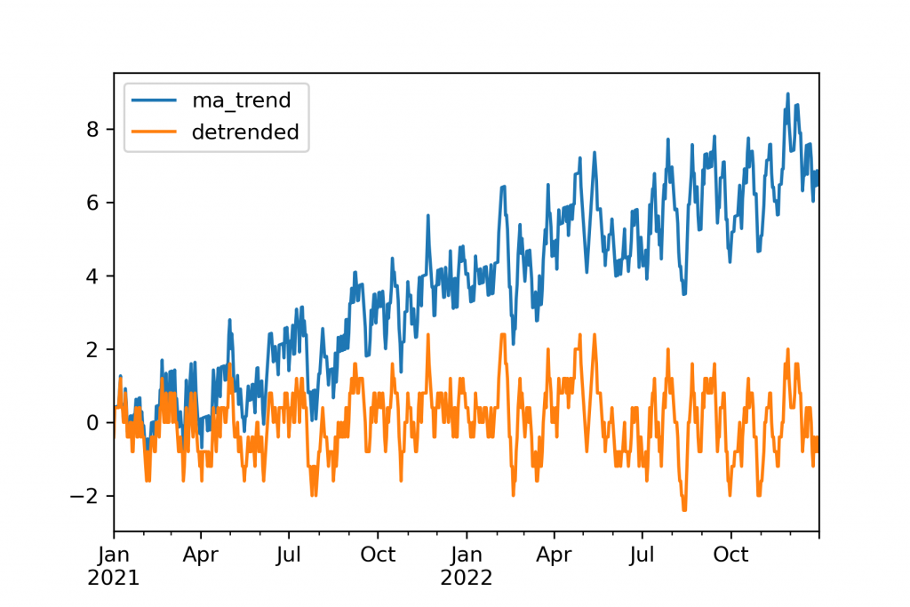
Time series specific preprocessing is then usually about separating signals. A decomposition is where a signal is handled by another method. For example, a detrending might use a linear regression to handle a secondary growth signal, then passing the data, without a trend, to be handled by the primary model. A filter is where signals are removed entirely. Most commonly this is a rolling mean or exponential rolling mean where each period becomes the average of that and several previous periods.

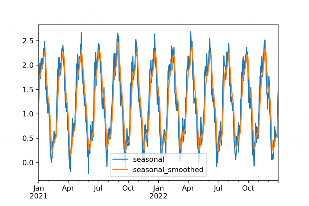
There is no single reason why these are to be used. Usually filters are used because models, especially machine learning models, will overfit, especially when too little history is available to show the signals true pattern. Often times they are advantageous simply because the output forecasts are then smoother and therefore more visually appealing than they might otherwise be. Decompositions are useful to handle signals that the downstream model will not handle as well. Some things, like PCA, are both a decomposition and a filter simultaneously.

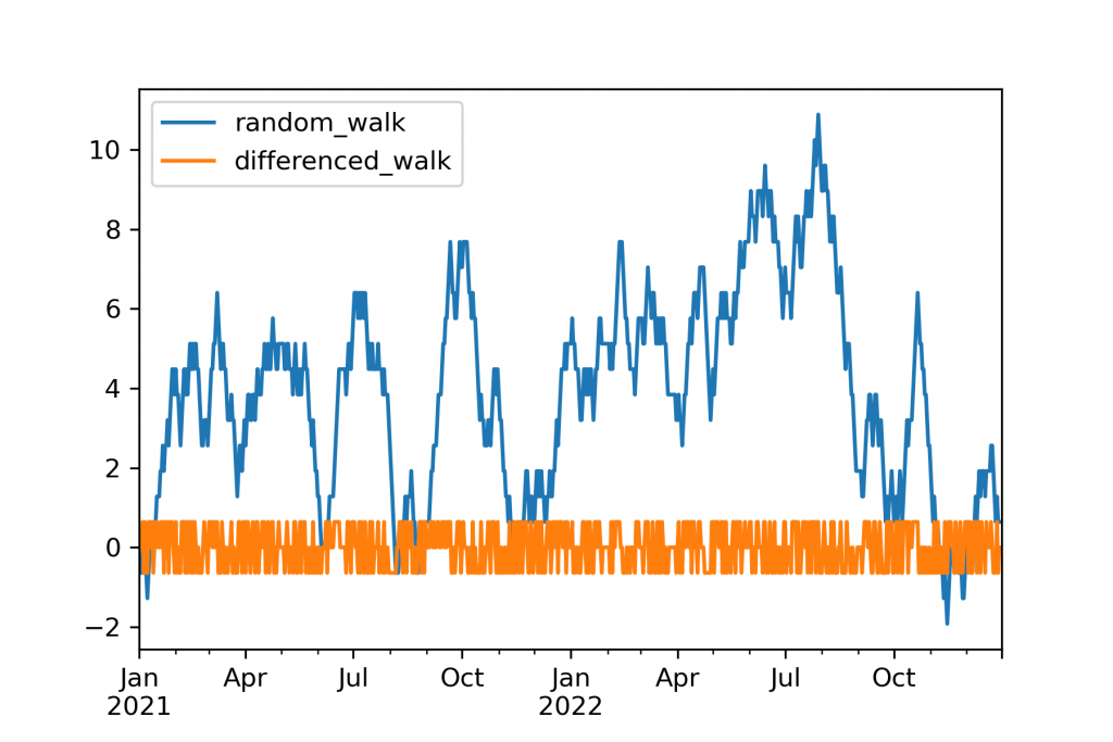
Finally, there are numerous transformations done simply to shift the data to better fit the assumptions of the model. A standard scaler as is used for many machine learning models can be used here, but there are additional transformations as well. Perhaps most well-known is differencing, subtracting the previous value from each period, used to remove the effects of a random walk before many models such as ARMA models.

A simple model, coupled with proper decompositions and filters, will almost always outperform a “more advanced” model.

The most important thing to remember, when using a transformation pulled in from the broader data science world, is to be very very careful about making sure it doesn’t transfer information backwards on the time series to past points from the future. This results in erroneously high accuracy, which won’t be repeated in a real-world test.

There is no one set of preprocessing steps that will work for all models and datasets. A few, however, are frequently valuable. Outlier removal and scaling (RobustScaler, MinMaxScaler, StandardScaler from scikit-learn) are sometimes helpful and usually a safe bet. I have also often found the QuantileTransformer to be useful. Differencing is helpful especially with traditional statistical methods which may require it. Finally, and often most valuably, is either rolling mean or exponential smoothing (.rolling() or .ewm() in pandas). Unlike the others, which require little or no parameter tuning, exponential smoothing may require some adjustment. Too little smoothing, and it won’t make a difference, too much smoothing and major signals may be lost.

Two example transformations are provided for the same real-world dataset. Both of these transformations are automatically-tuned, high-quality transformations. However, the output series are radically different. The data is monthly data for the Economic Policy Uncertainty Index for United States from FRED.

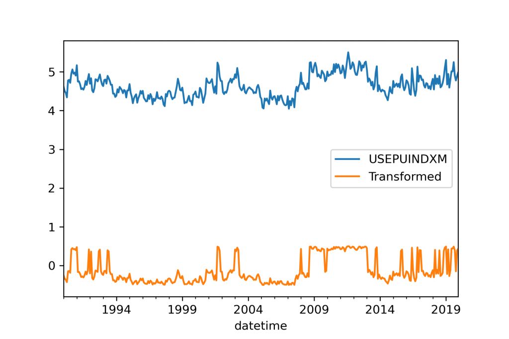
The first, using a Quantile Transformer and a Poisson detrending, has shifted the series to be around 0 and has emphasized the peaks in the dataset but generally retains the shape of the series. This was optimized for a machine learning forecasting model.

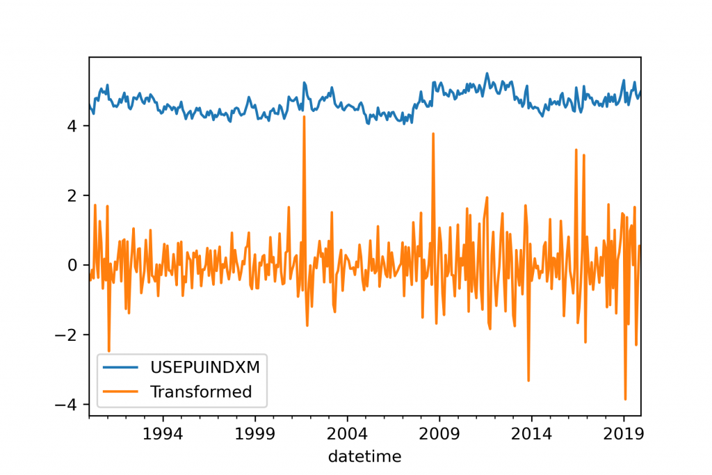
The second transformation here uses scaling, differencing, and linear detrending to produce a zero centered forecast that looks entirely different from the starting series. Experienced users will probably not be surprised that this was optimized for a statistical forecasting technique, as indeed the final output looks more like the ARMA processes that these models were usually designed for.

There are a couple of lessons from this exercise. The first is to realize that different models have different optimums for what preprocessing should be used. The second is that it can often be difficult to simply choose the optimal preprocessing by hand, and that searching for combinations across cross validation sets is important. Many data scientists don’t consider this aspect, tuning their model parameters but not their entire pipeline as a unit. AutoML packages can address this issue, using, for example, TPOT for machine learning generally, and AutoTS for time series forecasting specifically.

Hopefully this has been a helpful introduction to preprocessing for time series. Below is the sample for code for some of the plots used here.

import numpy as np
import pandas as pd


date_start = '2021-01-01'
date_end = '2022-12-31'
dates = pd.date_range(date_start, date_end)
size = dates.size
rng = np.random.default_rng()

df = pd.DataFrame({
    "random_walk": np.random.choice(a=[-0.8, 0, 0.8], size=size).cumsum() * 0.8,
    "ma_trend": np.convolve(
        np.random.choice(a=[-0.4, 0, 0.4], size=size + 6),
        np.ones(7, dtype=int),'valid'
    ) + np.arange(size) * 0.01,
    "seasonal": (
         (np.sin((np.pi / 7) * np.arange(size)) * 0.25 + 0.25) + 
         (np.sin((np.pi / 28) * np.arange(size)) * 1 + 1) +
         rng.normal(0, 0.15, size)
    ),
}, index=dates)

df['differenced_walk'] = df.random_walk - df.random_walk.shift(1)
# since the trend here is known, that is used, but otherwise a simple regression
df["detrended"] = df["arima007_trend"] - np.arange(size) * 0.01
df['seasonal_smoothed'] = df['seasonal'].ewm(span=7).mean()
df.plot()

from autots import GeneralTransformer, load_monthly
df2 = load_monthly(long=False)

out = GeneralTransformer(**{
    "fillna": "nearest", 
    "transformations": {"0": "StandardScaler", "1": "Detrend", "2": "DifferencedTransformer"},
    "transformation_params": {"0": {}, "1": {"model": "Linear", "phi": 1, "window": None}, "2": {}}}
).fit_transform(df2.USEPUINDXM.to_frame())
out.columns = ["Transformed"]
# log is used to make plot appear better on the same axis
df3 = pd.concat([np.log(df2.USEPUINDXM), out], axis=1)
df3.tail(360).plot()
plt.savefig("real_transformed1.png", dpi=300)

out = GeneralTransformer(**
    {"fillna": "time", "transformations": {"0": "QuantileTransformer", "1": "Detrend"},
     "transformation_params": {"0": {"output_distribution": "uniform", "n_quantiles": 100}, "1": {"model": "Poisson", "phi": 0.999, "window": None}}}
).fit_transform(df2.USEPUINDXM.to_frame())
out.columns = ["Transformed"]
df3 = pd.concat([np.log(df2.USEPUINDXM), out], axis=1)
df3.tail(360).plot()