
Demand forecasting is exactly how it sounds: forecasting demand. This can take many forms but the most classic example is predicting how many products will be sold by a retailer on each particular day. This forecasting is in turn used to drive business value in various ways. The most common is better inventory management, but also is often used for challenges like planning staffing and improving customer experience. Personally, I see potential for global benefit: better demand forecasting leads to more efficient energy use and less waste.
There are many difficulties in forecasting, of course, the crystal ball of the future is often cloudy. However here, I want to focus on one challenge in particular: intermittent demand forecasting. Intermittent forecasting is where the products being forecast are often zero, where the product just isn’t sold every day. Even at the warehouses of massive retailers, there are often a majority of products that don’t sell everyday.
Let’s look at why these are hard to forecast. For that I am going to use the dataset from a competition called the M5 competition. It’s a common baseline dataset in the literature and coming from Walmart is an excellent example of product demand. You can easily google this competition for more details. I start by using Prophet to model an example series from the dataset. Prophet is a very reliable time series model/package that is popular for good reason, it can consistently produce good (if not usually the absolute best) forecasts on many datasets.
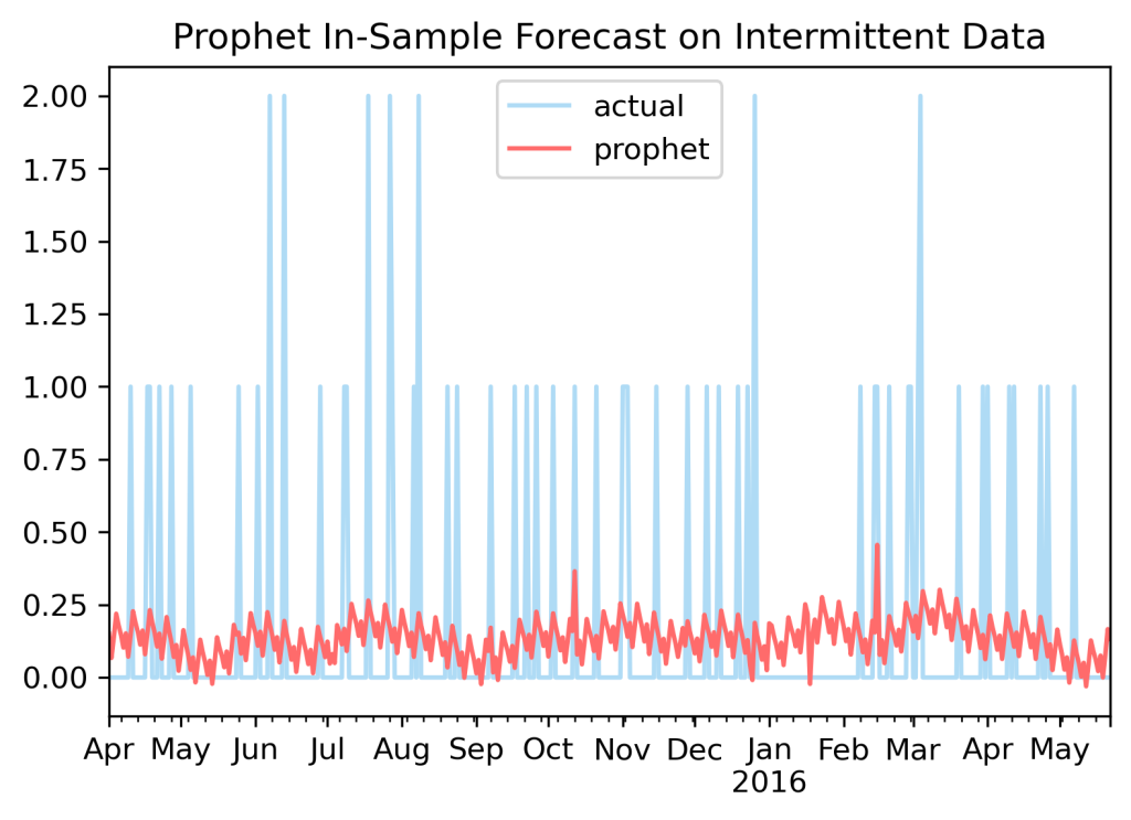
On this challenge, however, Prophet struggles. It is designed for series that ‘flow’ and here, all it runs into are a series of speed bumps. The Prophet forecast here, wavering between 0 and 0.2 for the most part, is not particularly useful. Many time series models were not designed to handle intermittent data, and even those that do, the classic approach is a two-part ETS approach called Croston, aren’t particularly admirable in their performance either.
As a quick note, intermittency can often be greatly reduced by aggregation. Instead of forecasting at the daily level, forecasting at a weekly or monthly level is often much easier. The sum across these periods of time is often no longer intermittent. A good solution, but not one that can always be used as daily level forecasts are often still required, so here we stay focused on the intermittent daily data.
The average data scientist’s approach to a problem is to throw more models and model parameter tuning at a problem to see if it solves the problem. This is not usually the right solution, but let us start with that. I am going to use AutoTS, a package I have written over several years to try to improve and fix all the problems of forecasting. Here AutoTS ran 38068 model and transformation parameter sets on 6 sampled series of the M5 competition dataset, starting from a previously optimized template. These took about 12 hours to run in total, including three total validations.
Here is the resulting forecasting, optimized on RMSE.
If you don’t know, RMSE, MSE, and SSE are three names for functionally identical* metrics, and these three are the most common metrics in regression problems in data science.
Note for advanced readers: I’ve also included a tiny SPL weighting in all model selections, to make sure the upper and lower forecasts weren’t too ridiculous in the graphs, not enough to significantly alter the point forecast, but probabilistic forecasts are a topic for another day.
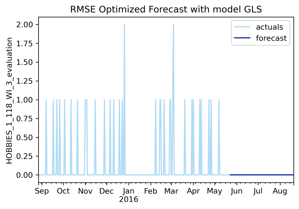
You are going to look at me and say, what is this rubbish? You have spent years optimizing this package, and it tried almost 40,000 models, and yet the best it could do was produce a flat line of just zero???
I do indeed get people saying exactly this to me sometimes. And, well yes, actually, the best it could do with this optimization task was a flat line.
See, RMSE strongly penalizes big mistakes, and with intermittent forecasting, all of your mistakes are big. Any time you predict something more than zero, it is fairly like to be wrong, that incurs a large error penalty, and so truly the best forecast on this series when target RMSE is a flat line of zeroes, which incurs the smallest overall error.
Now, one of the many cool things about AutoTS, when you are the author and know all the tricks, is you can utilize the evaluation metrics (it runs about 15 metrics by default right now) from all the ~38,000 models that were tried and select a new model that better fits a different criteria, without needing to run the entire search again for 12 hours.
Let’s try SMAPE instead of RMSE, a more forecasting specific metric and one that is quite popular because it is very easy to interpret across a large dataset. An SMAPE of 10 (sometimes presented as a decimal as 0.10, but AutoTS does the percentage) means that, on average, all series were off by 10%. It is the metric I would personally choose for reporting if I could only pick one.
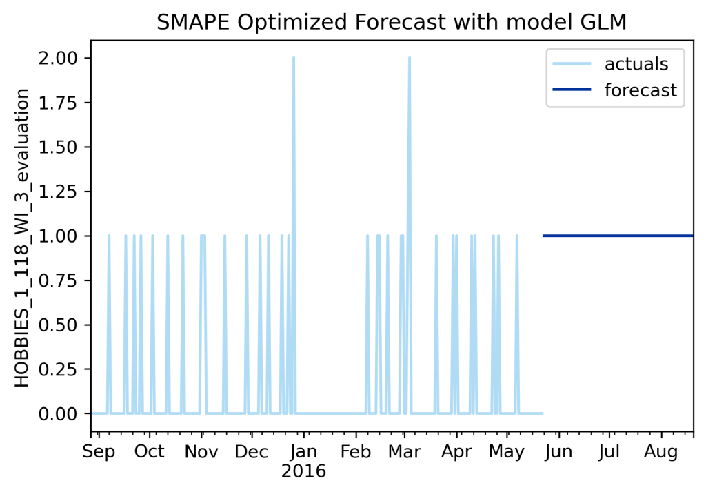
Still not looking to great, is it? Right, now we have another flat line. This one is predicting a constant value of ones. Fun fact, SMAPE doesn’t handle zeroes particularly well, and so ultimately favors all ones instead of all zeroes.
Now, I should step in here and say that sometimes the best you can do is some kind of flat line for the forecast. If the demand is really too random, and decently often it is, there is absolutely nothing better than a flat line of zeroes, or ones, or maybe 0.5, or whatever tests best in evaluation. But one thing I do know is that most clients/stakeholders hate receiving flat lines. They invested good money/time for something a kid could draw with a ruler?? So let us see if we can do better.
As I think you can see by how I have been leading you on, my focus here is going to be on evaluation criteria/metrics. Metrics aren’t the only thing that matter in making good forecasts, models and data preprocessing/transformers matter plenty, as does validation selection and so on, but the evaluation metrics really are the most important piece of the puzzle. The following discussion utilizes metrics new to AutoTS version 0.6.2 (except MAGE which has been around a while) and as of writing that is still in beta and not released (it should be out before Halloween 2023, in a week or so).
Let us try a new metric for forecast optimization: MAGE. This is named and created by me, and stands for Mean Aggregation Error. The concept is pretty simple: take the sum of all errors for all series across each day/period of the forecast. I originally created it to try and solve the problems of hierarchical forecasting by an approach of using cross validation results on a metric instead of all the other hierarchical nonsense people do.
Let’s understand it through a business case. Say you are a manager needing to decide how many stock pickers need to be in your warehouse today. The number of employees is directly proportional to the number of items to be picked. So you need an accurate number for total products to be shipped that day, but you don’t care as much about exact accuracy for each product forecast. Your most important goal is accuracy across all the sum of products. This is MAGE’s case. Take the sum of all forecasts of all products for the day and compare to the sum of all actuals for that day.
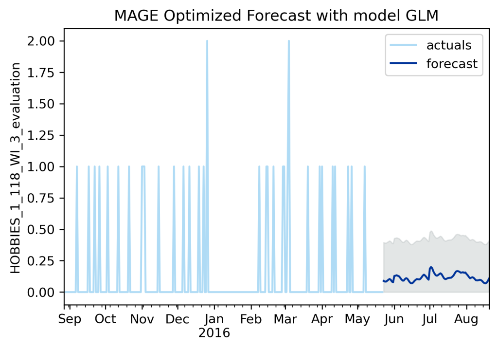
MAGE is starting to look a little better as an optimization metric. It is more than a flat line. It will do well on the overall aggregation. But… well, it still doesn’t really look great on an individual series, does it?
Let’s try something else. The following is MATE. MATE is Mean Absolute Temporal Error. It is MAGE but down the other axis, so instead of taking the sum across each time step, it takes the sum for each single product down the entire forecast time/horizon. The use case for this one is even easier to understand: you are managing inventory and are placing an order for inventory/stock every 90 days. You want your 90 day bulk purchase to be as accurate as possible for the total period being covered, but you don’t care as much about the accuracy on each particular day.

MATE looks much much better. I wouldn’t get too excited, I think it will sometimes optimize on a forecast that looks like MAGE too, mostly a flat line. Both of them care about overall and long term averages, so there is no strict requirement for a visual match of the nature of the series.
We cannot really stop at MATE and MAGE because while they work for long term averages they don’t have any concern about actual day to day accuracy, which we still care about for many use cases. The solution is the Wasserstein distance.
The Wasserstein or Earth Moving Metric looks at how much energy is required to reshape the predicted forecast into the actual data. Let’s say you generated a two day ahead forecast for some product. You predict: 0, 6. The actuals then turn out to be 6, 0 instead. Evaluating this with a conventional metric like RMSE would make this error look pretty bad. Both days are off by a value of 6, so 6^2 + 6^2 gives an RMSE of 72. Not a good forecast by RMSE standards. But the original forecast still looks promising, it predicted the right values, just not quite on the right day. Wasserstein distance looks at the energy required to move the forecast towards the correct value, and here, the error is not so large, because it is not so hard to move a value over one day. The actual math used involves a difference of the cumulative sums.
This metric will not work for all use cases. For example, for amusement park attendance forecasting, you need to have the right demand on the right day. You can’t say a big demand spike will occur on Friday when it actually falls on Saturday. You brought in all those extra staff for Friday that were bored and costing money for no need, then on Saturday the few staff brought in are overwhelmed and then customer and staff experience quality drops drastically. Indeed, this example is one case where RMSE is a better fit. Traditional metrics aren’t completely useless, they just shouldn’t be the only tool in your basket.
But for a quite a lot of demand forecasting use cases, like inventory management, being close, say within a day, is usually pretty good and within the tolerances of the system, making Wasserstein distance a good choice.
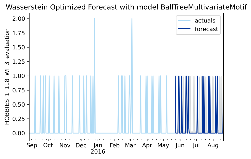
In this case, Wasserstein and MATE chose the same forecasts, so clearly the newly-introduced BallTreeMultivariateMotif model is looking promising. Actually I haven’t really tested how well that model scales to massive datasets, so don’t get too excited about it yet.
I would like to very briefly introduce one more set of potential metrics to you. These aren’t yet in AutoTS, and may never be, because they are too slow to calculate (at least, slow in the context of when you have to run them on each series for all 38,000+ models). They are distribution losses based on the distribution rather than the exact days of data (distribution as in a statistical distribution, not distribution as in ‘distribution center’). These provide a longer term view like MAGE or MATE rather than day-level accuracy, but unlike MAGE and MATE also enforce that the selection of values should match the actuals. In lay terms, these distribution losses will prefer a forecast of zeroes over a forecast of random wobbles (like Prophet) because at least one bin will be somewhat aligned, but they most strongly prefer a forecast that has spikes just like the spikes the actual series have, if not necessarily spikes at the same time as were observed.
The first approach to distribution loss is to make a histogram of the actuals and predicted, then calculate the chi-squared distance between the histograms. The second approach is to take a Kernel Density Estimator (KDE) on the data and then compare the forecast and actual KDEs by use of a metric like the KL Divergence.
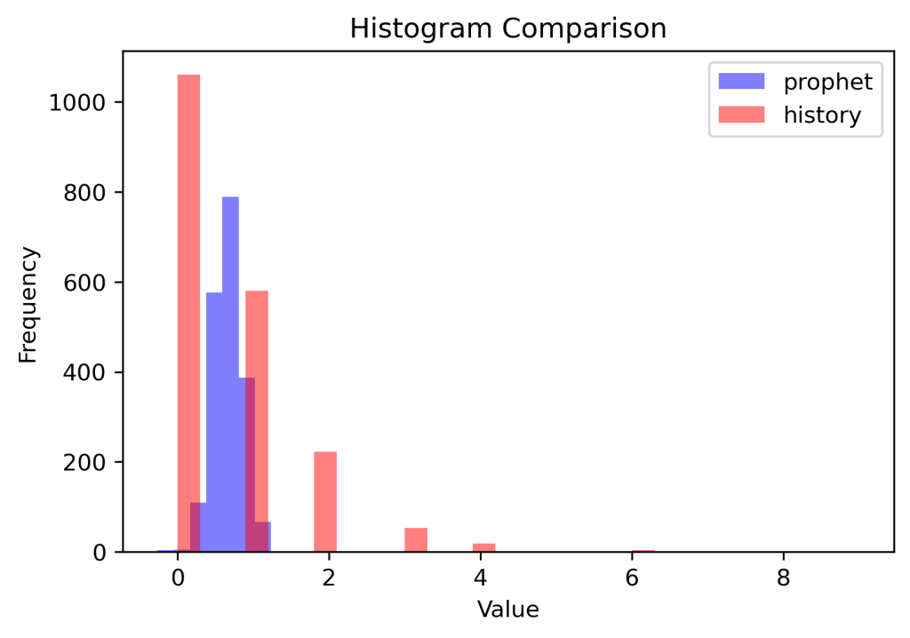
This image of the histogram of the earlier Prophet forecast at the start of the article against the histogram of actuals shows the values of this approach as well. It is instantly apparent that the forecast and actuals are fundamentally different and do not capture the same patterns. Useful for data scientist, yes, but these distribution loss metrics are a bit harder to tie directly into business uses cases than the other metrics.
There, enough, no more new metrics for you today.
The more observant of you may have noticed, especially in discussion of MAGE and MATE, that there was a better way to solve the use case offered as an example. Why not just forecast the one time series of total products for your staffing needs instead of forecasting each individual product and taking the MAGE accuracy of those? Well, actually, if you only had one use case, that staffing problem, you would probably do just that.
However, most forecasts in demand planning have multiple possible uses (staffing and inventory and shelf stocking) and you want a single master set of forecasts that can be used for all cases, because having 3 different official forecasts, one for each use case, is something managers hate, and with good reason, it is terribly confusing and may lead to conflicting decisions.
AutoTS enables you to solve multiple use cases at once, by passing a metric_weighting of a mix of different metrics. The goal is to balance the forecast selection criteria to choose one forecast that balances all of the needs as best as possible (perfect balance will usually be impossible). The below graph represents a mix of every metric discussed here, with small weightings for RMSE and SMAPE (because we want to try to get day to day precision like these offer, but don’t want to spend too much energy on it), then with the most weighting on MAGE, MATE, and Wasserstein (because these solve are actual uses cases best).
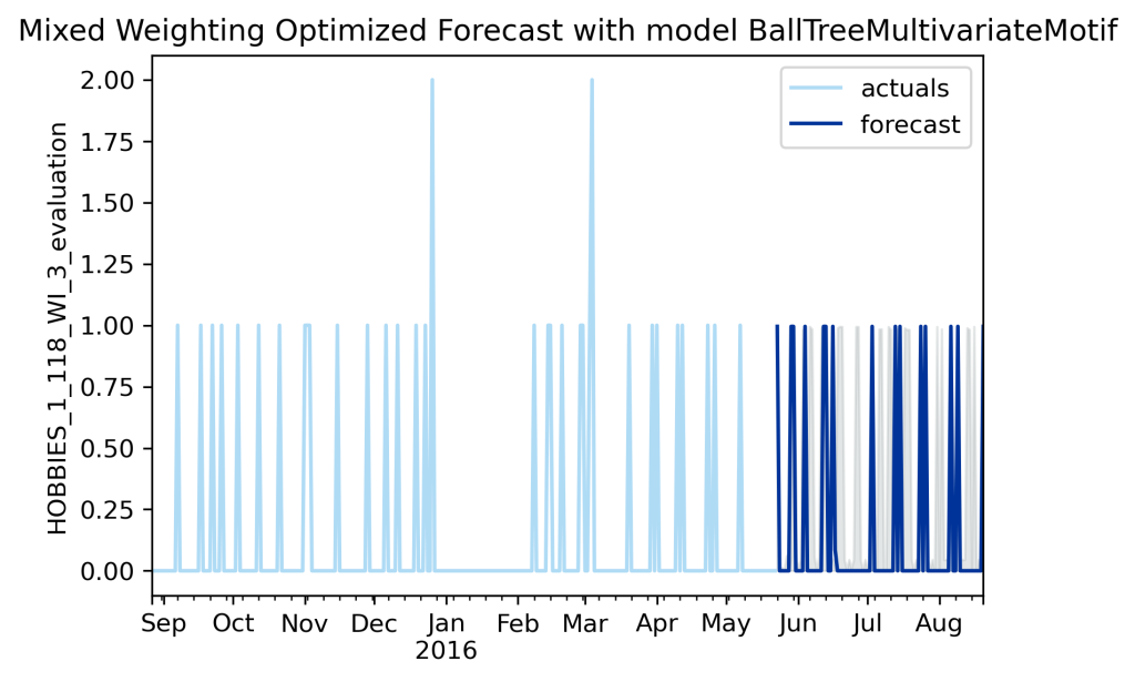
So it is a tiny bit boring because it makes the same forecast selection as the individual MATE and Wasserstein selections, but that is easy to change, a remix of the metric weightings yields different results.
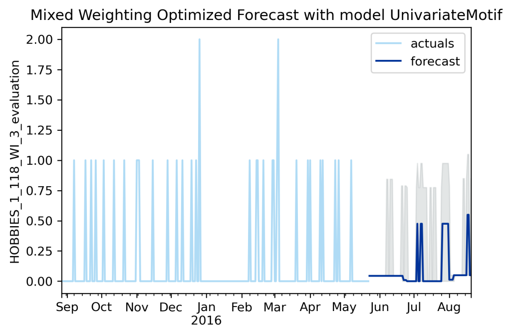
Above is a different mixed metric graph. I mixed these parameter weightings around (also adding in underestimate penalization) until I got something more unique. How do you choose what metric weighting to use? Well, it starts with the business use case: choose metrics that minimize the factors that most drive the value, plus important but less final value driven factors like ‘my manager hates flat lines so I need something wavy’. Then there is a bit of tinkering to get the exact weights balanced to capture the desired appearances (unfortunately AutoTS weightings aren’t quite perfectly balanced so sometimes values need to be a bit larger or smaller than you initially expect).
Let’s review the metrics and how they come together to make the one forecast to rule them all:
Your warehouse staffing needs an accurate demand expectation at the day level of how many products will need to be moved, but your staffing does not require an accurate day level forecast for each product. (This is MAGE)
Each product needs an accurate assessment of how much inventory is needed, but as purchases are occasional and in bulk, the long term aggregate demand for each product matters, not the day level of demand. (This is MATE)
However, leadership and product managers need to see forecasts that look like actuals. They need to see appropriately sized spikes, but their human eye won’t be able to see if those spikes fall quite exactly on the right day or not. Also, while we said we didn’t care about day level forecasting for inventory stocking, it would actually be really nice if the inventory demand fell on days as close as possible if not exactly on the right day. (This is Wasserstein) (variations on this might also benefit from distribution losses, directional accuracy metrics (DWAE/ODA), and shape fitting metrics (MADE/Contour))
Finally, it is still worth looking at exact day level precision across the full dataset, so RMSE, SMAPE, and others might still be included.
Personally, I see forecasting almost as triage. You cannot get perfect forecasts. Accordingly, your model selection and criteria needs to be focused on delivering what limited certainty can be found on the business value of the applied forecasting use case, even if that means it won’t be pretty. AutoTS makes this all easier and more accurate, but you can recreate the same metrics and processes elsewhere as well.
This is still an ongoing area of research. AutoTS is constantly being updated with new ideas. Keep an eye out for interesting new developments!
For code for these metrics, please checkout winedarksea/AutoTS on GitHub and view the autots/evaluator/metrics.py file.
# example weighting, untuned
metric_weighting = {
    'smape_weighting': 1,
    'rmse_weighting': 1,
    'spl_weighting': 1,
    'mage_weighting': 1,
    'mate_weighting': 1,
    'wasserstein_weighting': 1,
    'dwd_weighting': 1,
    'runtime_weighting': 0.05,
}